An LLM request looks simple from outside the cluster. A client sends a prompt, the service returns tokens, and a GPU does the work.
Inside the serving system, that request becomes two very different jobs.
First, prefill processes the input prompt and builds the key-value cache, or KV cache, that holds attention state for later tokens. Then decode generates one output token at a time while repeatedly reading that state.
Running both steps on one GPU is the simplest design. But it may become hard to scale.
Long prompts can delay requests that are already generating tokens. Decode-heavy traffic can use a lot of memory without using all available compute. A GPU pool sized for prefill may waste capacity during decode, or the reverse. The pool can look busy while still missing its latency targets.
Because the two steps need different resources, some inference systems now run prefill and decode in separate worker pools. Current systems including llm-d and NVIDIA Dynamo support this pattern. Recent research is already exploring finer splits across prefill, decode, attention, and feed-forward execution on heterogeneous hardware. A paper published on August 4, 2026 reported simulated throughput gains of up to 75% for prefill/decode disaggregation in its evaluated configurations, while stressing that the result depends on the model, hardware, and workload (Forys et al., 2026).
The extra worker pool is only part of the change. The network, worker placement, queues, and KV-cache location now affect whether each request is fast and correct.
One request, two different workloads
During prefill, the model processes the prompt tokens together. Each transformer layer performs large matrix operations, computes attention over the input, and writes keys and values into the KV cache.
This phase usually makes better use of parallel compute because there is substantial work available at once. Prompt length matters directly: more input tokens mean more prompt processing and a larger cache to produce.
Decode is different. The model generates a token, appends its new attention state to the cache, and then repeats the process for the next token. Each step depends on the previous step, so a single request exposes much less parallel work.
The decode worker also reads the existing KV cache on every generation step. As the number of active requests and their context lengths rise, memory capacity and bandwidth become central constraints. Batching helps by letting the GPU advance several requests together, but those requests finish, pause, or arrive at different times. The runtime must continuously rebuild the batch.
In simple terms:
- Prefill turns many input tokens into model state.
- Decode repeatedly reads that state to produce one token at a time.
The same accelerator can perform both jobs, but the best batch size, parallelism, capacity ratio, and scheduling policy need not be the same.
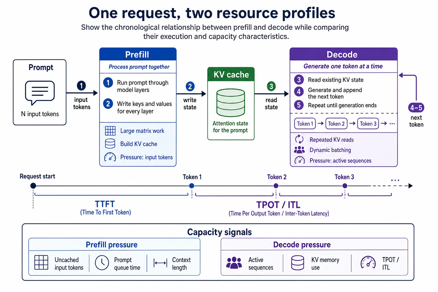
Prefill processes the prompt in parallel and creates the KV cache. Decode reads that state repeatedly while generating one token at a time.
TTFT and TPOT show the difference users feel
Users experience the two phases through different latency measurements.
Time to first token, or TTFT, measures the interval between sending a request and receiving its first token. It includes queueing, prompt processing, first-token generation, and network time in common client-side measurements (NVIDIA AIPerf metric definition).
Time per output token, often reported as inter-token latency or ITL, measures the average delay between tokens after the first one arrives. It represents the steady generation experience rather than the initial wait (NVIDIA NIM metrics).
This distinction matters during incidents. A service can have acceptable overall request latency while users wait too long for the first token. It can also start quickly but stream tokens too slowly for an interactive application.
For example, a queue of large document prompts may primarily damage TTFT. Too many concurrent long generations may primarily damage TPOT. If both phases share one pool, the first problem can create the second: large prefills occupy execution time that active decode requests need to maintain a smooth token cadence.
Do not rely on averages alone. Track at least p50 and p99 TTFT and TPOT, split by input length, output length, model, cache-hit class, and route. Otherwise, a large population of short requests can hide the tail behavior of the requests that drive capacity.
Why one GPU pool becomes hard to tune
An aggregated worker runs prefill and decode in the same process and on the same accelerator allocation. This has useful properties: no remote KV handoff, fewer components, and a small failure surface.
The tradeoff is interference.
Suppose an interactive coding service is already decoding hundreds of requests. A new request arrives with a 50,000-token repository context. Its prefill needs substantial compute and creates a large KV cache. The runtime can prioritize that prompt, split it into chunks, or make it wait. Each choice moves latency somewhere:
- Running the prefill immediately can interrupt decode progress and increase TPOT.
- Delaying it protects active generations but raises TTFT.
- Dividing it into chunks reduces blocking but adds scheduling complexity and may still consume capacity needed by decode.
Replica-level autoscaling does not fully solve this. Adding identical workers scales both capabilities together even when the workload needs more of only one. A traffic shift from long-input summarization to long-output reasoning can reverse the required ratio without changing the request rate much.
This is where the case for separate pools begins.
Separate worker pools change capacity planning
In a disaggregated deployment, a prefill worker processes the prompt and creates its KV state. A decode worker then receives or accesses that state and continues generation.
The pools can scale independently. You can also give them different tensor-parallel layouts, batch limits, cache allocations, or accelerator types. Dynamo explicitly supports separate scaling and configuration for the two phases, and its design allows different parallelism choices for prefill and decode (Dynamo design documentation).
This creates a more useful capacity model:
- Prefill demand follows arrival rate, uncached input tokens, and prompt complexity.
- Decode demand follows active sequences, generated tokens, context length, and token-rate targets.
- The handoff tier follows KV bytes transferred per second, transfer concurrency, and topology.
That last line is easy to miss. Once the pools are separate, available GPU capacity is not enough. The system also needs enough transfer capacity to connect them.
A good autoscaling policy therefore needs phase-specific signals. Prefill queue depth and waiting input tokens can drive prefill scaling. Active decode sequences, pending decode tokens, KV utilization, and observed TPOT can drive decode scaling. A single GPU-utilization target will often react late or scale the wrong pool.
Now the network is part of inference
The KV cache is not a small request header. Its size grows with the number of layers, cached tokens, attention configuration, and cache data type. Moving it between workers puts a potentially large transfer directly between prompt processing and token generation.
That transfer can erase the benefit of disaggregation if the data path is slow. NVIDIA’s current Dynamo guidance treats fast KV movement as an early deployment requirement and warns that a TCP fallback can let transfer time dominate TTFT and throughput in cross-node deployments (Dynamo disaggregated serving guide). Its NIXL-based design supports direct GPU-to-GPU movement over available transports such as NVLink or InfiniBand/UCX (Dynamo design documentation).
For an infrastructure team, this creates several new operational concerns.
Placement: A free decode GPU across a slow topology boundary may be a worse target than a busier GPU near the prefiller. Dynamo now supports topology-aware routing intended to keep KV transfers within a rack, zone, or another labeled domain (topology-aware KV transfer).
Backpressure: A prefill worker should not keep admitting prompts if their caches cannot be transferred or accepted by decode workers. Otherwise, completed prefills accumulate state while user-visible progress stops.
Retries: Retrying prefill after an ambiguous handoff can duplicate expensive work. Retrying decode on another worker may require another KV transfer. The request protocol needs identifiers and clear ownership so the system knows whether cache state exists and whether it is safe to reuse.
Failure domains: A prefill crash, decode crash, transfer timeout, or router restart fails the request at a different point. llm-d’s disaggregation documentation calls out additional network hops, stranded memory after prefill failure, and the need for timeout and retry handling (llm-d disaggregation design).
Tail latency: Median transfer time is not enough. Queueing on a shared fabric, a cross-rack route, or a transport fallback will appear in TTFT. Measure the full handoff, including time waiting for the destination to reserve cache blocks.
Treat the transfer path as a service dependency. Give it latency and throughput objectives, dashboards, saturation alerts, and failure injection tests.
The router now makes important decisions
A normal load balancer can choose a healthy endpoint with a short connection count. A disaggregated inference router needs to make a placement plan.
It may consider:
- How many prompt tokens are not already cached?
- Is the prompt large enough to justify remote prefill?
- Which worker has matching prefix state?
- Which decode worker has enough KV memory?
- How deep is each phase’s queue?
- Can the selected pair exchange KV data over a fast path?
- Will this placement meet both TTFT and TPOT targets?
llm-d’s router evaluates prefix-cache locality and worker load, and its disaggregation handler can skip remote prefill for short prompts or prompts with a strong cache match on the decode worker (llm-d router documentation). Its precise cache-aware configuration can consume actual KV-block events and combine cache residency with queue and cache-utilization signals (llm-d cache-aware routing guide).
That conditional path is important. The production choice is not necessarily “always aggregated” or “always disaggregated.” It can be a per-request decision.
A short prompt may run entirely on a decode worker because a remote handoff costs more than the prefill it avoids. A long uncached prompt may go to a specialized prefill pool. A prompt with a large cached prefix may follow that cache even if another worker has a shorter queue.
The scheduler is therefore making latency and capacity tradeoffs, not merely balancing requests. Its decisions should be observable. Record the chosen workers, cache score, queue score, topology domain, disaggregation decision, KV bytes, transfer duration, and fallback reason in a request trace.
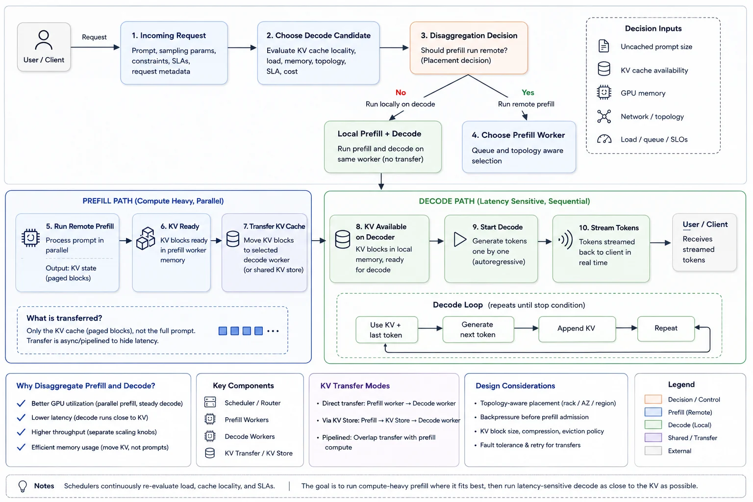
A useful router does not split every request. It weighs saved prefill work against cache locality, queueing, and KV-transfer cost.
When separate pools help—and when they do not
Disaggregation is most promising when the phases have clearly different pressure and the deployment has enough traffic to use separate pools efficiently.
Good candidates include:
- Long-input retrieval, document, or coding workloads
- High-concurrency services with strict token-streaming targets
- Mixed workloads whose input/output ratios change over time
- Large models that benefit from different parallel layouts by phase
- Clusters with a fast, observable GPU-to-GPU transfer fabric
It may be a poor fit when:
- Prompts are short and remote transfer exceeds saved prefill time
- Traffic is too low to keep both pools useful
- The model fits comfortably on a small aggregated worker
- Prefix reuse already lets decode workers avoid most prompt computation
- Cross-node networking is slow, congested, or operationally opaque
- The team cannot yet trace and benchmark the extra request stages
Recent research supports this conditional view rather than a universal rule. The August 2026 HeteroPanacea paper found large simulated gains in some configurations, but those gains varied with model architecture and assumed hardware specialization (Forys et al., 2026). Dynamo’s deployment guidance likewise says aggregated serving may remain simpler and faster for small models, short prompts, low concurrency, or clusters without fast KV transfer (Dynamo user guide).
The right comparison is not GPU utilization in isolation. It is goodput: requests completed within the TTFT and TPOT targets that matter to the application.
Build the baseline before you split the pool
Start with an aggregated deployment and a replayable workload. Capture the real distribution of input tokens, output tokens, concurrency, prefix reuse, and service-level targets. Then test disaggregation against exactly the same traffic.
Measure these stages separately:
- Router queue time
- Prefill queue and execution time
- Decode reservation time
- KV transfer setup, bytes, and duration
- First-token generation time
- Steady-state TPOT
- Fallbacks, retries, and failed handoffs
Run at least three layouts: aggregated, always disaggregated, and selective disaggregation. The selective policy should initially be simple, such as a threshold based on uncached prompt tokens. Complexity can come later.
On Kubernetes, keep the serving runtime responsible for model execution and KV movement, while the platform handles placement, health, rollout, and resource isolation. Systems such as llm-d combine Kubernetes Gateway API integration, cache-aware routing, and specialized worker roles; its published P/D guide provides a concrete deployment shape for teams that want to test the pattern (llm-d P/D guide).
Do not begin by buying separate hardware for each phase. First prove that the resource mismatch exists and that the transfer path can preserve the latency you intend to gain.
Splitting prefill and decode turns one hard capacity problem into several smaller ones. You can scale each step separately, but every request must now cross a distributed system.
The next step is to run a benchmark. Use real traffic, set separate TTFT and TPOT targets, and compare one GPU pool with a selective split. Count KV transfer, queue time, failures, and idle capacity. If the split still wins, you have evidence that the extra system complexity is worth it.
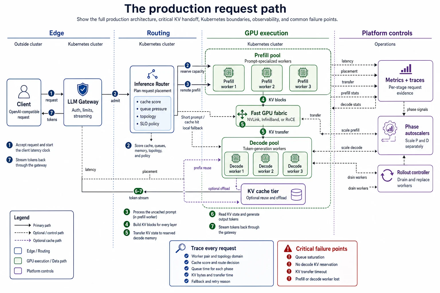
After disaggregation, the model runtime is only one part of the serving path. Routing, admission, KV movement, topology, and fallback behavior determine whether the split works.
Sources
- When Does Disaggregation Pay? Simulating Prefill--Decode--Attention--FFN Specialization for Agentic LLM Inference — Recent research on prefill/decode and operator-level specialization, including simulated throughput results and workload-dependent limits.
- Disaggregated Inference Serving in llm-d — llm-d request lifecycle, worker selection, conditional disaggregation, cache-aware decisions, and stated operational limitations.
- llm-d Router — Current llm-d routing architecture, Endpoint Picker role, cache-aware placement, load signals, and Kubernetes Gateway integration.
- llm-d Prefill/Decode Disaggregation Guide — Concrete Kubernetes deployment guide for llm-d prefill/decode disaggregation.
- llm-d Precise Prefix Cache Aware Routing Guide — Use of real KV-block events, prefix residency, queue size, and cache-utilization signals in placement.
- NVIDIA Dynamo: Disaggregated Serving — Independent worker pools, scaling pressure, KV transfer requirements, RDMA guidance, suitable workloads, and cases where aggregation is preferable.
- NVIDIA Dynamo Disaggregated Serving Design — Three-step request flow, direct GPU-to-GPU KV transfer, worker routing, and phase-specific parallelism.
- NVIDIA Dynamo: Topology-Aware KV Transfer — Routing prefill and decode within rack, zone, or other topology domains to reduce slow transfers.
- NVIDIA AIPerf Metrics Reference — Definitions and formulas for time to first token and inter-token latency.
- NVIDIA NIM LLM Benchmark Metrics — Operational definitions of TTFT and ITL/TPOT and the effect of prompt processing on TTFT.